A benchmark for Monte Carlo simulation applied to gamma-ray spectrometry
The use of Monte Carlo (MC) simulation in gamma-ray spectrometry is getting more and more interest since it can be run on PCs. Such approach is useful to perform different kinds of calculation, such as efficiency calibration, efficiency transfer or coincidence summing corrections.
In the frame of the Gamma Spectrometry Working Group (GSWG) of the International Committee for Radionuclide Metrology (ICRM), a benchmark has been prepared, as a learning tool for the use of Monte Carlo codes applied to gamma-ray spectrometry.
There are two kinds of software which can be used for these. The dedicated codes (GESPECOR, DETEFF, etc.) are conceived with a user-friendly interface and can be directly applied to derive the calculation results from input data. On the contrary, the use of generalist codes (GEANT4, MCNP, PENELOPE, etc.) need some training in order to derive the information of interest. One of the typical difficulties is the preparation of the input files which describe the geometrical conditions, since these must be written according to a specific format. To facilitate the use of generalist MC simulation software, the ICRM GSWG participants prepared geometrical files for a selection of high-purity germanium detectors (HPGe) and measurement conditions, and computed the total and full-energy peak efficiency for five energies. For each code, a specific information form, the input files and the results are available in the archives: GEANT4, MCNP, PENELOPE, EGSnrc.
The first part of the exercise was presented during the ICRM 2019 conference and the summary of the results was published (A benchmark for Monte Carlo simulation in gamma-ray spectrometry, M.C. Lépy, C. Thiam, M. Anagnostakis, R. Galea, D. Gurau, S. Hurtado, K. Karfopoulos, J. Liang, H. Liu, A. Luca, I. Mitsios, C. Potiriadis, M.I. Savva, T.T. Thanh, V. Thomas, R.W. Townson, T. Vasilopoulou, M. Zhang, Applied Radiation and Isotopes 154 (2019) 108850, https://doi.org/10.1016/j.apradiso.2019.108850).
The full report including all results is available there.
A second part of the exercise is underway; it is devoted to the calculation of the coincidence summing corrective factors. As for the first part of the exercise, the participant were asked to calculate the coincidence summing corrective factors for the eight geometrical study cases for some radionuclides with typical decay schemes: 60Co and 134Cs are beta minus emitters, 133Ba decays by electron capture and is characterized by intense X-ray emission, while 22Na decays by both electron capture and beta plus emission, the latter leading to the emission of annihilation photons. The results were presented during the last ICRM conference in Bucharest and are published.
Benchmark files
The ICRM GSWG participants contributed to prepare benchmark files specific to four different MC codes (EGSnrc, GEANT4, MCNP and PENELOPE). Two cases have to be considered since GEANT4, which is object-oriented and run under UNIX, must be compiled including the geometry, while the other codes are written in FORTRAN and run with an external geometry file.
The exercise was based on the simple models which were defined by Vidmar in an exercise dedicated to coincidence summing corrections (see annex 1). Geometry models include a detector and a source with different combinations; however, in all the cases, a complete cylindrical symmetry of the arrangement of sample and detector is assumed. Two kinds of coaxial HPGe detector are considered. For both, the active crystal of the detector consists of a germanium cylinder with a thickness and diameter of 60 mm, with a 40-mm depth hole of 10-mm in diameter. It is installed in a 1-mm thick aluminium housing, with a length and diameter of 80 mm, and the crystal-to-window distance is 5 mm. The only difference between the two models is the dead layer thickness (on the top and side of the crystal), that is 1 mm or 0 mm to simulate either a p-type detector (“Detector A”) or a n-type one “Detector B”. One point source and 3 volume sources are considered, each been located at 1 mm from the detector window. No source containers are to be simulated and the volume sources are cylinders made of water (Diameter 90 mm – thickness 40 mm), silicon dioxide (Diameter 60 mm – thickness 20 mm) and cellulose (Diameter 80 mm – thickness 3 mm) with respective density 1.0, 1.4 and 0.3. The last two sample models are supposed to reproduce the case of soils and filters measuring conditions. These sources are respectively denoted “P”, “W”, “S” and “F” in the exercise.
Each source-detector assembly is installed in a 50-mm thick lead shielding, which has both a diameter and a height of 400 mm. The characteristics of various materials to be used in the simulation of the detector and sample models were also provided according to Vidmar (2014). On the whole, eight configurations (2 detectors x 4 sources) are considered, using the following “names” to identify each geometry:
| Name | Detector | Source |
| AP | A | Point |
| AW | A | Water |
| AS | A | Soil |
| AF | A | Filter |
| BP | B | Point |
| BW | B | Water |
| BS | B | Soil |
| BF | B | Filter |
Figure 1 shows an example of the p-type detector in combination with the water source (without the external shielding).
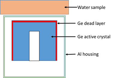
Figure 1: Geometrical model for the case of water source with p-type detector (“AW” case).
The participants prepared input files specific to the MC code they are familiar with, and computed the full-energy peak efficiency (FEPE) and the total efficiency (TE) for five energies (50 keV, 100 keV, 200 keV, 500 keV and 1 MeV), for the eight combinations.
Results:
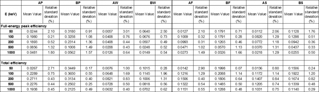
Table 1 summarizes the mean values obtained by the participants, and the relative standard deviation of the results. In most of the study cases presented here, the relative standard deviation is less than 1 %, nevertheless, one can notice some discrepancies, especially for the 50-keV incident photons. In fact, there are different approaches either in the implementation of the physical interaction processes or in the practical definition of the efficiencies which prevent from achieving full comparison between the Monte Carlo codes.
Table 1: Mean value and standard deviation of the participants results for the eight study cases
Equivalence of computer codes for calculation of coincidence summing correction factors
(From: Vidmar, T., Capogni, M., Hult, M., Hurtado, S., Kastlander, J., Lutter, G., Lépy, M.-C., Martinkovic, J., Ramebäck, H., Sima, O., Tzika, F., Vidmar, G., 2014. Equivalence of computer codes for calculation of coincidence summing correction factors. Applied Radiation and Isotopes 87, 336–341.)
Instructions for participants
A set of well-defined detector and sample geometries is considered. In all the cases, a complete cylindrical symmetry of the sample-detector geometry is assumed. The parameters of the two simulated closed-end coaxial HPGe detectors, a p-type and an n-type one, are given in Table 2, and a sketch of the p-type detector in combination with a point source is also provided (Figure 2). The two detectors are identical, except for the thickness of their respective dead layers. The sample parameters are given in Table 3. No source containers are to be simulated in this step. In the calculations, the sources should all be placed at a distance of 1 mm from the detector window.
A cylindrical lead shielding should also be included in the simulations. It has both a diametre and a height of 400 mm and its thickness on all sides is 50 mm. The detector is placed centrally within the lead shielding, with the central points of the shielding itself and of the detector crystal coinciding. This leaves a gap of 110 mm between the detector housing and the lead shielding on all sides.
The characteristics of various materials used in the constructions of the detector and sample models are given in Table 4.
Table 2: Detector parameters. All dimensions and given in millimetres (mm).
The housing diameter is in all cases the same as the window diameter.
| Parameter | Detector A | Detector B |
| Crystal material | Ge | Ge |
| Crystal diameter (including the side dead layer) | 60 | 60 |
| Crystal length (including the top dead layer) | 60 | 60 |
| Dead layer thickness (top and side) | 1 | 0 |
| Hole diameter | 10 | 10 |
| Hole depth | 40 | 40 |
| Window diameter | 80 | 80 |
| Window thickness | 1 | 1 |
| Window material | Al | Al |
| Crystal-to-window distance | 5 | 5 |
| Housing length | 80 | 80 |
| Housing thickness | 1 | 1 |
| Housing material | Al | Al |
Table 3: Sample parameters. All dimensions and given in millimetres (mm).
| Parameter | Water | Point | Soil | Filter |
| Sample diameter | 90 | – | 60 | 80 |
| Sample thickness | 40 | – | 20 | 3 |
| Sample material | Water | – | Dirt | Cellulose |
| Sample-to-window distance | 1.0 | 1.0 | 1.0 | 1.0 |
Table 4: Characteristics of various detector and sample materials.
All densities are given in g/cm3.
| Material | Density | Chemical formula |
| Ge | 5.323 | Ge |
| Al | 2.70 | Al |
| Water | 1.0 | H2O |
| Dirt | 1.4 | SiO2 |
| Cellulose | 0.3 | C6H11O5 |
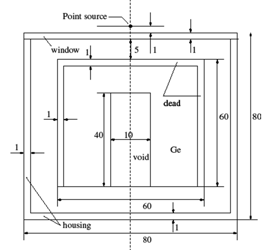
Figure 2: A schematic presentation of the setup for the case of the point source and the p-type detector model.